
Twenty years ago AWS launched a service so simple they named it after the premise: just put a file in and get it back out. Today that service holds 500 trillion objects. The name never changed. The service became something else entirely. Most people are still using it like it’s 2006.
Today that service holds 500 trillion objects. It handles 200 million requests per second. The price has dropped roughly 85% since launch to just over two cents per gigabyte, while almost every other cloud cost has gone up. The name has not aged as well as the service.
Here is what no one tells you when you start: S3 is not the hardest part of AWS storage. The hardest part is that AWS storage is not one thing. It is a collection of services that look superficially similar, have overlapping use cases, and were built by different teams over different decades. When you open the AWS console and see EBS, EFS, FSx, S3, S3 Glacier, S3 Express, S3 Tables, S3 Vectors, and Storage Gateway all listed as “storage services,” you are not confused because you are doing something wrong. You are confused because it actually is confusing.
This guide is about building the mental model that makes it stop being confusing. Not a tour of every setting and configuration option; that is what the AWS documentation is for, and it is terrible at building intuition. This is about understanding what each service actually is, why it exists, when to reach for it, and what the wrong choice costs you.
Start here. Come back to the documentation when you know what you are looking for.
What Storage Actually Is
Before any AWS-specific discussion, we need to agree on some fundamentals, because almost every wrong storage decision traces back to a confused picture of what storage even is.
There are three fundamentally different things people mean when they say “storage.”
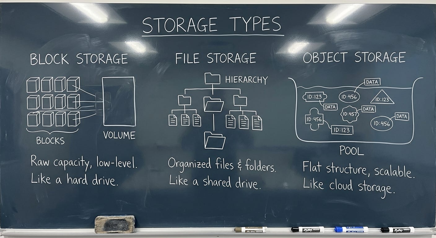
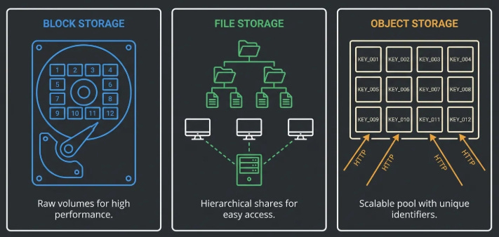
Block Storage
Think about the hard drive in your laptop. Your operating system sees it as a sequence of numbered blocks, tiny fixed-size chunks of space, each with an address. The OS writes data by filling in those blocks. It keeps a separate table (the filesystem) that records which blocks belong to which file, where each file starts and ends, and so on. The drive itself knows nothing about files. It just stores blocks and hands them back when asked.
That is block storage. Raw, low-level, fast. The OS and the applications on top of it are what turn those blocks into something meaningful.
This matters for AWS because one of AWS’s core storage services, EBS, is exactly this: a managed block device. It behaves like a hard drive that you plug into a server. Your database writes to it. Your operating system boots from it. It is fast and flexible because the software on top can use it however it wants. It is also constrained, for the same reason: only one machine can use a block device at a time (with narrow exceptions we’ll get to), because having two machines simultaneously writing to the same raw block device is a coordination nightmare that most software is not built to handle.
File Storage
Now imagine that hard drive lives in a dedicated server, and instead of plugging it directly into one machine, you expose it over the network. Multiple machines can connect to it simultaneously and interact with it through a shared filesystem. Same directories, same files, same folder structure, all visible to everyone connected.
This is file storage, also called network-attached storage or NAS. The protocol that most Linux and Mac systems use to connect to a network filesystem is called NFS, which stands for Network File System. Windows systems typically use SMB, which stands for Server Message Block. The names are irrelevant, the concept is: a shared filesystem over a network.
AWS has multiple services in this category (EFS, FSx). They exist for the same reason on-premises NAS exists: some applications were built to work with a shared filesystem and cannot easily be redesigned. A rendering cluster where fifty machines all need to read and write to the same asset library needs file storage. A legacy enterprise application that expects a drive letter mapped to a network share needs file storage.
Object Storage
Object storage is the weird one. It does not look like a disk. It does not look like a filesystem. It looks like a giant key-value store accessible over HTTP.
A key-value store is exactly what it sounds like: you give it a key (a name), it gives you back a value (the thing you stored). You PUT a key-value pair in, you GET a value back by providing the key. That is the entire interface. There are no directories. There are no folders. There are no blocks. There is no concept of appending to an existing value or changing part of it. You write the whole thing, or you read the whole thing.
When S3 shows you a “path” like my-bucket/images/2024/photo.jpg, that is not a directory tree. There is no folder called images. There is no folder called 2024. That entire string — images/2024/photo.jpg — is a single key. The slashes are cosmetic. S3 uses them to simulate a folder interface in the console because humans are more comfortable with folders, but underneath there are no folders. There is just a flat list of keys.
Why does this matter? Because the object storage model is what makes the scale possible. A filesystem needs a server to maintain state: who has which file locked, what does the directory tree look like, where does each file start and end on disk. That server is a single point of coordination. As it grows, it gets slow. As it gets slow, everything waiting on it gets slow. This is why on-premises NAS gets creaky at scale.
Object storage has no single coordinating server. Every object is independent. You can spread billions of objects across thousands of machines with no coordination needed, because nothing depends on anything else. Want to add a machine? Add it. Want to lose a machine? Replace it. The objects just get redistributed. This is how you get to 500 trillion objects. And it is also why you cannot append to an S3 object or write to a specific byte offset in place, there is no server maintaining that kind of mutable state. Byte-range reads are a different matter: S3 fully supports them, and they are a key performance pattern for reading portions of large files without downloading the whole thing. The limitation is on writes, not reads.
If you find yourself constantly fighting the “I can’t just write a few bytes to S3” constraint, you are using the wrong storage type. That is not a bug in how you are using S3. That is the signal that you need a database or block storage.
The Decision Tree: Which Service, When?
Here is the thing about the AWS storage decision: it is not as hard as it looks, because most of the options are for specific situations that you will know when you are in.
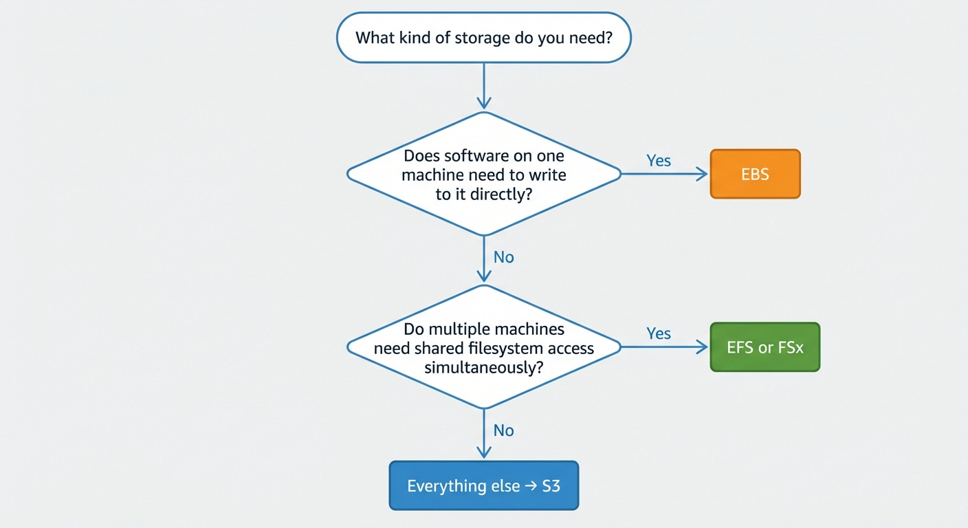
Start by asking three questions in order.
First: does your data need to be attached to one specific compute instance and modified in place by software running on that instance?
If yes, that is EBS. Your database lives here. Your OS disk lives here. Your application’s local scratch space lives here. EBS is a managed block device that attaches to one EC2 instance (EC2 is AWS’s virtual machine service, more on that in a different issue) and behaves exactly like a hard drive. You do not share it. You do not access it over HTTP. You plug it in and your software uses it as a disk.
Second: does your application need multiple machines to access the same data simultaneously through a shared filesystem?
If yes, that is EFS or FSx, depending on what kind of filesystem you need.
EFS (Elastic File System) is managed NFS for Linux. Multiple EC2 instances, across multiple data centers, can mount it at the same time and see the same directory tree. It scales automatically. You pay for what you actually use, not what you provision. It is the right answer for shared application state, content management systems, development environments, and any Linux workload that was built assuming a shared filesystem exists.
FSx is a family of managed filesystem services for more specific needs. FSx for Windows File Server speaks SMB and integrates with Active Directory, the directory service that Microsoft environments use to manage users and permissions. This is the service for Windows workloads that need network shares.
FSx for Lustre is a high-performance parallel filesystem (“parallel” meaning it can feed data to hundreds of compute nodes simultaneously at very high throughput), designed for scientific computing and ML training.
FSx for NetApp ONTAP is a managed version of a popular enterprise NAS product called NetApp, notable right now because it can expose file data through S3’s interface, letting AI services read your NAS data as if it were object storage. More on that when we get to the AI section.
Third: is your data in neither of those categories?
Everything else belongs in S3. Backups. Media files. Data lakes. Model training datasets. Log archives. Static websites. Application build artifacts. Anything that you write once and read many times, or anything you send to users over the internet, or anything you want a data analytics service to query, S3 is the answer.
This is not a default-to-S3-because-it-is-familiar answer.
It is a the-object-storage-model-is-actually-correct-for-most-use-cases answer.
The data you think you need a filesystem for usually does not actually need a filesystem. It needs durable storage and HTTP access. That is S3.
The cost difference reinforces this. EFS costs roughly $0.30 per GB per month. S3 Standard costs $0.023 per GB per month. That is thirteen times more expensive for EFS. If your application can be redesigned to use S3 without requiring filesystem semantics or low-latency in-place mutation, the economics are strongly in favor of doing so.
S3 Is Four Different Services Now
This is where most guides fall behind. They describe S3 as one service with a lot of settings. That was true in 2019. It is not true now.
There are four distinct bucket types in S3. They have different performance characteristics, different durability guarantees, different pricing, and different use cases. Choosing between them correctly saves money and prevents performance problems. Choosing wrong means either overpaying or building something that hits a wall.
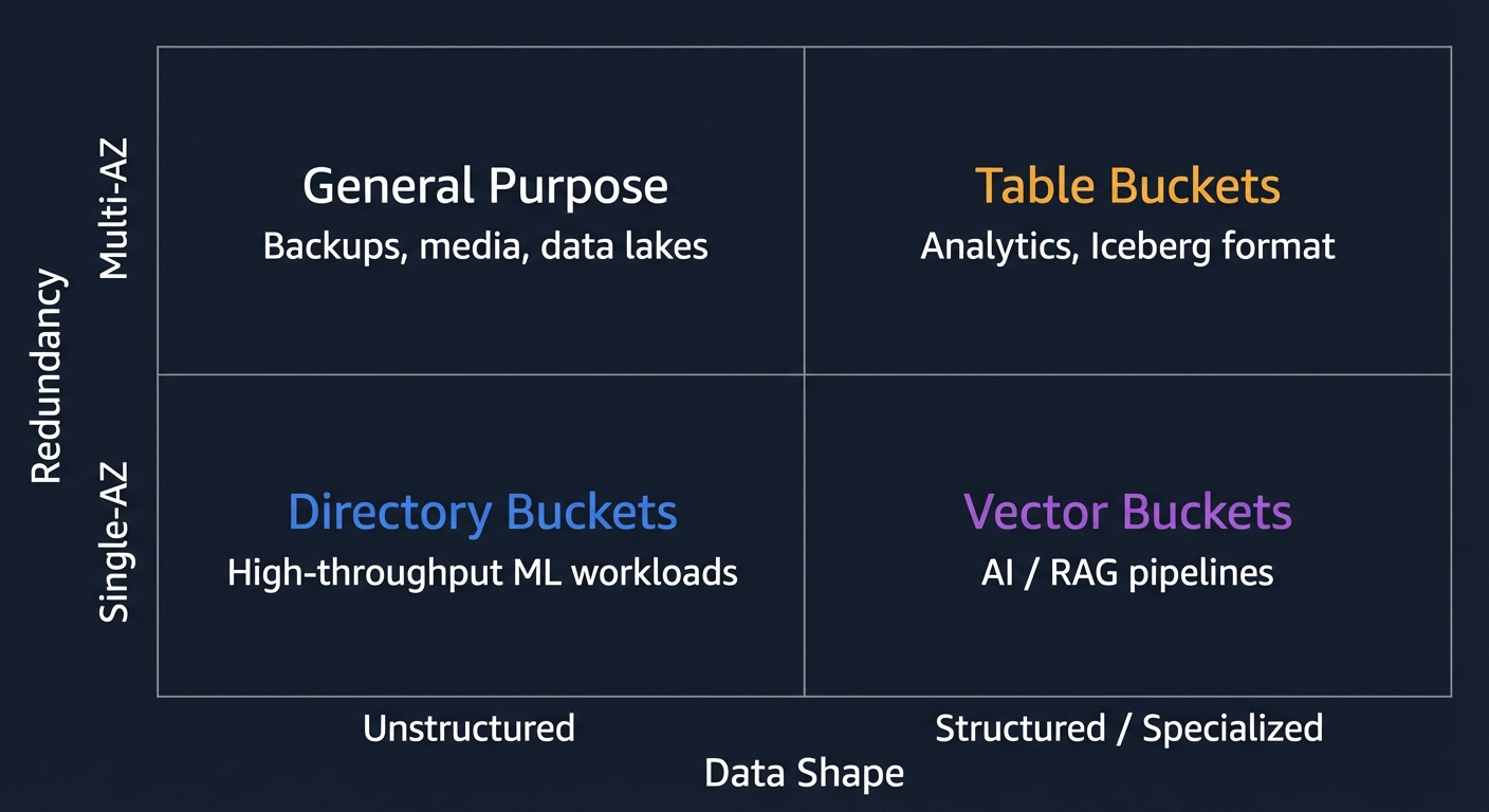
General Purpose Buckets
This is the original S3. When someone says “S3,” they almost certainly mean this. Understanding it well is the foundation for everything else.
Objects in a general purpose bucket are stored redundantly across at least three Availability Zones. An Availability Zone, or AZ, is AWS’s term for a physically separate data center within a region. A region is a geographic area — like US East (Northern Virginia), or EU West (Ireland). Within each region there are multiple AZs, each in a separate building, with separate power, separate networking, and enough physical distance between them that a flood, fire, or power failure that takes out one AZ is unlikely to affect another.
Why does this matter? Because S3’s 11 nines of durability (99.999999999%) is achieved by storing every object in three AZs simultaneously. If one entire data center burns down, your objects are still in two others. You would have to lose three separate data centers simultaneously to lose data, and if that happens, AWS has bigger problems than your files.
The consistency model deserves a paragraph because a lot of people are operating on outdated information. Before December 2020, S3 used something called eventual consistency for overwrites and deletes. Eventual consistency means: you write a change, and for some period of time afterward, some reads might return the old version. It was maddening to work around. People built retry loops. People added five-second delays. People kept separate records of what they had just written.
AWS fixed it in December 2020. S3 is now strongly consistent for all operations. You PUT an object, you immediately GET the new version. You DELETE an object, you immediately no longer see it in LIST results. There is no propagation window. If you are still writing code that works around eventual consistency in S3, you can delete that code. It is doing nothing.
One recent addition worth flagging: Account Regional Namespaces. Bucket names in S3 are globally unique across all AWS accounts. If someone else has already registered my-company-prod, you cannot have it, anywhere in the world. Account Regional Namespaces lets you reserve a bucket name pattern exclusively for your account by appending a unique suffix. It is enforced via IAM policies. IAM, or Identity and Access Management, is AWS’s permission system, which we will cover in the permissions section. The practical effect: you can stop losing bucket name races.
Cost check: Standard storage is $0.023 per GB per month in us-east-1. Not the number to fixate on. The number to fixate on is egress, what it costs when data leaves S3 to the internet. More on that later.
Directory Buckets (S3 Express One Zone)
General purpose buckets store data across three AZs. Directory buckets store data in one AZ. In exchange for that reduction in redundancy, you get dramatically better performance: consistent single-digit millisecond latency for frequently accessed data and up to ten times higher write throughput.
“Single-digit millisecond” sounds like marketing language, but it is actually a meaningful distinction. AWS documents S3 Express One Zone as up to 10x faster than S3 Standard with consistent single-digit millisecond latency. For most applications the latency difference does not matter. For ML training jobs trying to feed data to hundreds of GPU instances as fast as possible, it is measurable overhead that costs you money in compute time. Directory buckets close that gap.
The tradeoff is real: single AZ means you trade multi-AZ resilience for single-AZ placement and performance. Data is stored redundantly across multiple devices within that AZ (AWS designs it for 99.95% availability) but an AZ-level outage would make your data inaccessible until the zone recovers. AWS has not lost a complete AZ, but it is a real risk to model. For training data that exists elsewhere, or for intermediate results you can regenerate, this is an acceptable tradeoff. For data that is the only copy of anything important, it is not.
Directory buckets introduce hierarchical directory semantics; unlike general purpose buckets, directories are first-class concepts optimized for traversal rather than simulated with slashes. The path prefix/subdir/file.txt behaves like a directory hierarchy for indexing and performance purposes. It is still object storage, not a POSIX filesystem, but the directory-aware structure is what enables the higher throughput: operations that depend on prefix locality are faster when directories are real rather than cosmetic.
Cost check: Requests cost more per API call than general purpose buckets. Model your total workload cost (storage plus requests) before assuming this is cheaper than general purpose.
Table Buckets
Here is where S3 starts doing things its creators did not anticipate.
Table buckets store data in Apache Iceberg format. If you have not encountered Iceberg before: it is an open standard for storing large datasets on object storage in a way that makes them queryable like a database table. The name “Apache” indicates it is an open-source project maintained by the Apache Software Foundation, which is a nonprofit that stewards a lot of foundational open-source software.
Here is what Iceberg actually is, because “table format” is not a self-explanatory phrase.
When you store a lot of data in S3, you typically store it as Parquet files. Parquet is a file format optimized for analytics; it stores data in columns rather than rows, which means if you want to compute the average of one column across millions of rows, you can read just that column without reading the rest of the data. That is fast and efficient.
The problem: Parquet files are just files. S3 does not know anything about what is inside them. If you want to query all of them, you have to scan every file. If you want to find all records where a certain field equals a certain value, you have to read everything. And if two processes are writing to your dataset simultaneously, or if you want to see what the data looked like yesterday, you have no way to do that. Parquet is a file format, not a database.
Iceberg adds a metadata layer on top of Parquet files that tracks: what files are in the dataset, what the schema looks like, how the data is partitioned (more on that in a moment), and the full history of every change ever made to the dataset. With this metadata, Iceberg can do things a raw set of Parquet files cannot: ACID transactions, which means writes either fully succeed or fully fail with no partial states visible to readers; schema evolution, meaning you can add or remove columns without rewriting all the data; time travel, meaning you can query the dataset as it existed at any point in the past; and partition pruning, meaning when you query for records matching a filter, Iceberg can figure out which files could possibly contain matching records and skip the rest.
“Partition” is the data concept worth pausing on. When you have billions of records, scanning all of them for every query is slow and expensive. Partitioning means organizing the data into groups based on a column value; typically something like date or region — so that queries filtered by that column only need to read the relevant group. A query for “all records from January 2024” reads only January 2024’s partition, not all of 2020, 2021, 2022, and 2023.
Before Table Buckets, using Iceberg on S3 required managing an external catalog — typically AWS Glue, which is AWS’s managed metadata catalog service — to keep track of the Iceberg metadata. Table Buckets move that management into S3 itself. You get a managed Iceberg table that integrates natively with Athena (AWS’s SQL query service for S3 data), Glue, and Redshift (AWS’s data warehouse service), without external catalog setup.
Table Buckets now support Intelligent Tiering (the automatic tier-shifting system we will discuss in the next section) with up to 80% cost savings for infrequently queried data, and cross-region replication.
The AWS VP of S3 called Table Buckets one of the two most significant API-level changes in the service’s twenty-year history. That is a high bar. The justification: S3 Tables move Iceberg table management (compaction, snapshot cleanup, catalog maintenance) into S3 itself. Before this, you had to orchestrate that maintenance manually or through Glue jobs. Athena and Glue are still part of the picture for querying and catalog integration, but the operational burden of keeping the Iceberg catalog consistent with the actual data is now AWS’s problem, not yours.
Cost check: Table Buckets cost more per GB than general purpose buckets. The correct comparison is not “S3 Standard vs S3 Tables” but “S3 Tables plus Athena query costs vs Redshift Serverless for the same analytical workload.” At meaningful scale, S3 Tables is often significantly cheaper than a managed warehouse.
Vector Buckets
The newest bucket type. Purpose-built for AI workloads, specifically for something called RAG; Retrieval-Augmented Generation.
Here is what RAG is, because it is worth understanding before discussing the storage layer.
Large language models; the category of AI that includes the models behind Claude, GPT, and others, learn patterns from training data but cannot update their knowledge after training. If you ask a language model trained in early 2024 about something that happened in late 2024, it does not know. If you ask it about your company’s internal documents, it does not know. The model’s knowledge is frozen at training time.
RAG is the technique for getting around this. The idea: at query time, before sending the user’s question to the language model, retrieve relevant documents from your own knowledge base and include them in the prompt. The model now has access to information it was never trained on. It can use that context to give accurate, up-to-date, organization-specific answers.
The retrieval step is where vector search comes in. You cannot just search for documents that contain the user’s exact words, because users do not always use the exact words that are in the documents. You need semantic search, finding documents whose meaning is similar to the question, even if the wording is different.
The way this works: a separate model called an embedding model converts both documents and queries into lists of numbers (vectors) that capture semantic meaning. Documents about similar topics end up with similar numbers. The question “how do I reset my password?” and the document “account recovery steps” produce vectors that are numerically close to each other, even though they share no words. Finding the closest vectors to a query vector is called nearest-neighbor search.
Vector Buckets store those vectors and run the nearest-neighbor search natively. The numbers: up to 2 billion vectors per index, 10,000 indexes per bucket, query latency under 100 milliseconds for frequently accessed data. AWS claims this is up to 90% cheaper than running a dedicated vector database like Pinecone.
The use case is specifically read-heavy RAG workloads; you generate embeddings once, store them, and query them repeatedly. S3 Vectors supports metadata filtering natively, by default all metadata attached to vectors is filterable, so you can combine similarity search with attribute filters in a single query. Where OpenSearch becomes the better choice is when you need hybrid search (combining vector similarity with full-text keyword search), aggregations, faceted search, or very high query throughput where you need sub-100ms latency consistently rather than the ~100ms warm query latency S3 Vectors delivers. Vector Buckets are the right default for new RAG pipelines where simplicity and cost matter.
Cost check: No minimum floor. You pay per query and per GB stored. Compare against OpenSearch Serverless, which requires at least two indexing compute units at roughly $700 per month before you store a single document.
General Purpose S3: The Full Picture
The rest of this section is about general purpose buckets, because they are what you will use most of the time and there is a lot of it to understand.
Storage Classes and the Lifecycle Machine
S3 Standard is not the only place to put objects in a general purpose bucket. There is a tiered system of storage classes, and understanding them is worth real money at scale.
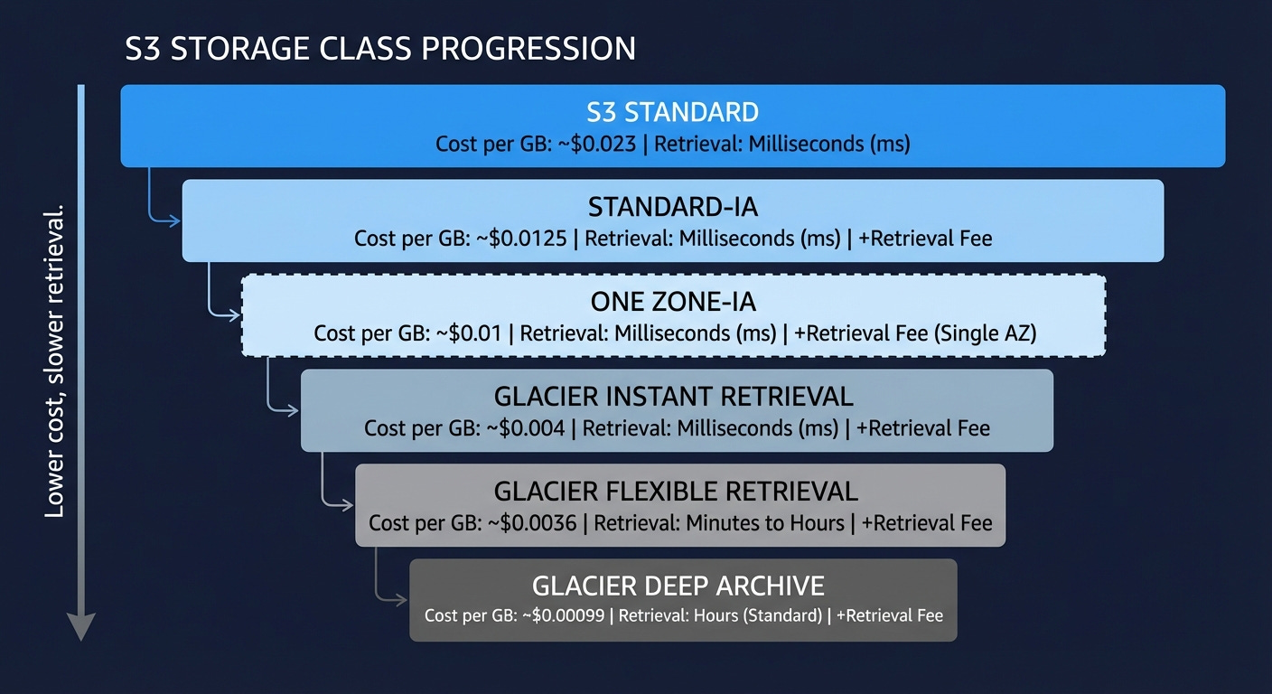
The underlying logic is simple: data ages. Objects you created yesterday get read constantly. Objects you created three years ago get read almost never, but you still need them. Storing both at the same price is wasteful. AWS created storage classes to let you pay less for data you access less, with the tradeoff being either higher retrieval costs, longer retrieval time, or both.
S3 Standard is the starting tier. Full redundancy across three AZs, millisecond retrieval, no minimum storage duration, no retrieval fee. You pay the full storage rate. Use this for anything you access regularly.
S3 Standard-Infrequent Access (Standard-IA) has the same three-AZ redundancy and millisecond retrieval as Standard, but lower storage cost in exchange for a per-gigabyte retrieval fee. There is also a 30-day minimum storage duration charge, meaning if you put something in and delete it after a day, you still pay for 30 days. And a 128 KB minimum object size charge, so small objects get charged as if they were 128 KB. The math tips in your favor when you access data less than roughly once a month. Good for disaster recovery copies, infrequently accessed backups, and secondary datasets.
S3 One Zone-Infrequent Access is the same pricing model as Standard-IA but stored in a single AZ. Twenty percent cheaper on storage. If that Availability Zone has an outage, the data becomes unavailable until the zone recovers. It is not replicated across AZs, so this tier should only be used for data you can recreate. Use it for generated derivatives: transcoded video variants, image thumbnails, processed outputs, where the original source exists in a more durable location.
S3 Glacier Instant Retrieval is where you cross from “infrequent access” into “archival” territory. Retrieval is still milliseconds, but storage is significantly cheaper than Standard-IA, and the minimum storage duration jumps to 90 days. The retrieval fee is higher than Standard-IA. Use this for data you access roughly once a quarter or less.
S3 Glacier Flexible Retrieval trades retrieval speed for cost. You have three retrieval options: Expedited (1 to 5 minutes), Standard (3 to 5 hours), and Bulk (5 to 12 hours). Bulk retrievals are free. This is the right tier for backup archives and long-term data retention where you can tolerate waiting hours for access when you need it.
S3 Glacier Deep Archive is the cheapest storage AWS offers. Retrieval time is 12 hours minimum. You put something here when you are legally required to keep it but do not realistically expect to ever read it. Financial records held for regulatory compliance. Medical records past their active retention period. Anything where the access scenario is “audit, not operation.”
A note on naming confusion: S3 Glacier also exists as a separate, older service with its own API, predating the storage class model. If you encounter Glacier vault operations in legacy code or old documentation, that is the original standalone service. For anything new, use the S3 storage classes. They are cheaper to operate, simpler to manage, and integrated with everything else in S3. The standalone Glacier API is effectively superseded.
The Lifecycle Machine is how you automate movement between these tiers. You define rules: move to IA after 30 days, move to Glacier Instant after 90 days, move to Deep Archive after 365 days, delete non-current versions after 7 days. These rules run automatically with no application changes. Set them once and your data self-manages its cost profile as it ages.
The savings on a large dataset can be substantial. A petabyte that ages from Standard through to Deep Archive over a year costs dramatically less than a petabyte that sits in Standard forever because nobody got around to setting up lifecycle rules. Do the math for your data. Then set the rules.
One trap practitioners learn expensively: S3 lifecycle rules operate on object creation date, not last access date. S3 does not track last access time by default. A rule that says “move to Glacier after 90 days” will move an object 90 days after it was created, regardless of whether it was read yesterday. If you have a bucket full of objects created two years ago that your application reads daily, a 90-day lifecycle rule will tier them immediately and generate retrieval fees every time they are accessed. Before setting age-based lifecycle rules on any bucket, verify whether the objects are actually accessed infrequently. S3 Inventory combined with server access logs, or Storage Lens request metrics, will tell you. If access patterns are unpredictable, Intelligent Tiering is the right tool precisely because it makes tiering decisions based on actual access behavior rather than age.
Intelligent Tiering
Intelligent Tiering is a storage class that monitors object access patterns and moves objects between tiers automatically, with no retrieval fees. The tiers are Frequent Access, Infrequent Access (after 30 days without access), Archive Instant Access (after 90 days), and optionally Archive Access and Deep Archive (at 90 and 180 days respectively, though these require manual retrieval).
The catch is the monitoring fee: $0.0025 per 1,000 objects per month. That is not much per object, but it accumulates. For a bucket with 100 million small objects: log lines, sensor readings, event records, the monitoring fee can exceed the storage savings. Intelligent Tiering is cost-effective when your objects are larger than roughly 128 KB and your access patterns are genuinely unpredictable. If you know your access patterns, explicit lifecycle rules are cheaper and simpler. If you genuinely do not know which objects will get accessed and when, let Intelligent Tiering figure it out.
Object Naming and Partition Performance
Here is a problem that does not exist until you are at scale, and then it is urgent.
S3 distributes object storage internally across partitions — shards, roughly speaking — based on key prefixes. A key prefix is just the leading portion of your object key. For a key named logs/2024/01/15/server1/request-12345.json, the prefix might be logs/ or logs/2024/ depending on how many objects share that leading string.
The relevance: S3 supports at least 3,500 write requests and 5,500 read requests per second per prefix. If all your objects share the same prefix and you are generating more than 3,500 writes per second, you will start getting throttled with 503 SlowDown errors. S3 scales up automatically over time, but the auto-scaling takes minutes, and if you have a sudden write burst, you hit the limit before the system catches up.
The fix for workloads that consistently need throughput above these limits: spread your keys across multiple prefixes. Add a hash or random component at the start of the key. Instead of logs/2024/01/15/file.csv, use a3f/logs/2024/01/15/file.csv where a3f is derived from a hash of the filename. With ten distinct leading characters, you effectively have ten times the available throughput because each character prefix is an independent partition.
For most workloads (anything below millions of requests per minute) this is unnecessary complexity. If you see 503 SlowDown errors, this is the fix. If you are not seeing them, do not add the complexity preemptively.
Multipart Uploads
Objects uploaded in a single PUT request have a maximum size of 5 GB. For anything larger, you use the multipart upload API. AWS recommends using it for anything over 100 MB. The maximum size of a single S3 object via multipart upload is 5 TB. If you are storing large database dumps, video masters, or ML model weights approaching that ceiling, plan accordingly.
The concept is what it sounds like: break the object into parts (each between 5 MB and 5 GB), upload them in parallel, then tell S3 to assemble them. Advantages: parallelism makes large uploads faster; a failed part can be retried without restarting the entire upload; the upload can be paused and resumed across sessions.
The hidden trap: incomplete multipart uploads cost money. If your application starts a multipart upload and then fails before calling the “complete” API, because of a crash, a network error, a bug, the parts stay in your bucket and you pay for the storage indefinitely. They are invisible in the console unless you specifically look for them. A bucket with years of failed multipart uploads can accumulate surprising costs.
The fix is a lifecycle rule that expires incomplete multipart uploads after a reasonable period: seven days is a common choice. AWS exposes this as a native lifecycle rule type. Set it on every bucket where you are doing multipart uploads. It takes two minutes and it will eventually save you money.
The Permissions Layer Cake
S3 has four overlapping mechanisms for controlling access: Block Public Access settings, Bucket Policies, IAM policies, and ACLs. Before explaining what each one does, it is worth explaining why there are four of them, because it looks like overengineering until you understand the history.
ACLs (Access Control Lists) are the original mechanism, dating to the earliest days of S3. An ACL is a list attached to each object and bucket specifying who can do what: read, write, read the ACL itself, write the ACL, full control. They operate on AWS account IDs and a few predefined groups (like “all authenticated AWS users” or “public internet”). They were built before IAM existed, and they show their age. They are a legacy mechanism. Unless you are integrating with a system that specifically requires ACLs, turn them off. Set Object Ownership to “Bucket owner enforced” in your bucket settings. This is now the default for new buckets created after April 2023.
IAM policies are the main way permissions work in AWS. IAM stands for Identity and Access Management. The idea: every entity in AWS, a human user, an application, an EC2 instance, has an IAM identity. You attach policies to those identities that define what they are allowed to do. An EC2 instance running your application gets an IAM role that allows s3:GetObject on your specific bucket. The application running on that instance can then read from the bucket. The policy is attached to the identity.
Bucket Policies are the resource-side counterpart. Instead of attaching a policy to an identity, you attach it to the bucket itself. A bucket policy can grant or deny access to any principal; identities from your own account, identities from other AWS accounts, specific IP address ranges, or conditions like “only if the request comes from within a VPC.” Bucket policies are the right tool for cross-account access, for enforcing that all access must use encrypted connections, and for making specific paths publicly readable.
Block Public Access is a safety net. It is a set of settings at the account level and bucket level that prevent public access from being granted, regardless of what the bucket policy says. If Block Public Access is on and your bucket policy says “public read allowed,” Block Public Access wins. It was built because too many organizations accidentally made their buckets public and exposed sensitive data. Enable it at the account level by default. Disable it only for specific buckets that genuinely need to serve public content.
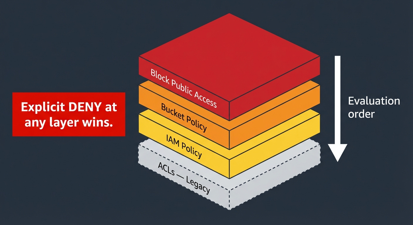
The precedence rule is the most important thing to understand about all four layers: an explicit Deny always wins, from any layer. If your IAM policy denies an action, a permissive bucket policy does not override it. If your bucket policy denies an action, a permissive IAM policy does not override it. When you cannot figure out why access is being denied, do not look for missing Allows first, look for explicit Denies at every layer. That is almost always the answer.
One more mechanism worth understanding: presigned URLs. A presigned URL is a time-limited URL for a specific object, signed with the credentials of the signer. Anyone who has the URL can access that object for the duration of the expiration window, regardless of the object’s own access settings. No AWS credentials required on the client side.
This is the standard pattern for sharing S3 objects with users who do not have AWS accounts: your backend generates a presigned URL and gives it to the client, the client uses it to download directly from S3.
The expiration limit depends on how you generate the URL. Console-generated presigned URLs max out at 12 hours. URLs generated via the CLI or SDK can be set up to 7 days. The catch: if you sign the URL using temporary credentials, which includes any Lambda function or EC2 role using an IAM role, which is essentially everyone, the URL expires when the underlying credentials expire, regardless of what expiration you specified. A Lambda-generated presigned URL set to 7 days will expire in hours because the Lambda’s session token is short-lived. To get URLs that actually last days, you need to sign them with long-term IAM user credentials, which introduces its own key management headache. Design your expiration windows to match what your credential type can actually deliver, a URL that expires before the client finishes downloading is a support ticket.
Versioning and the Versioning Tax
Versioning keeps every historical version of every object. When you overwrite an object, S3 does not replace it; it creates a new version and the old one persists alongside it. When you delete an object, S3 inserts a delete marker, but the previous versions remain. You can retrieve any previous version by specifying its version ID.
This is genuinely useful for compliance, accidental deletion recovery, and audit history. It is also a silent cost multiplier that nobody warns you about.
Imagine an application that generates a JSON status file every minute: dashboard data, configuration state, whatever. The file is 10 KB. With versioning enabled, every minute produces a new version and the previous minute’s version persists. That is 1,440 versions per day, about 525,000 per year, totaling roughly 5 GB of stored version history for a 10 KB file. Multiply that across ten files, or a hundred, and you have a problem.
The fix is lifecycle rules for non-current versions. Define what “keep” means for your situation (the last 5 versions, the last 30 days, the last 1 year) and set a lifecycle rule that deletes older versions automatically. Without this rule, versioning is a cost sink that grows forever. With it, versioning does what you want at predictable cost.
Object Lock is the compliance extension of versioning. It enforces WORM semantics (Write Once, Read Many) meaning once an object is written, it cannot be deleted or overwritten for a defined retention period. Two modes: Governance mode, where users with special IAM permissions can override the lock; and Compliance mode, where nobody can override it, including the root account. If you are in a regulated industry (finance, healthcare, legal), and you have records that must be immutable by law (SEC 17a-4, HIPAA, and various other regulations specify this), Object Lock is the right tool. It requires versioning to be enabled on the bucket.
Encryption
Every object in S3 has been encrypted at rest by default since January 2023. The question is not whether to encrypt (that is not a choice anymore) but which key management model to use.
SSE-S3 (Server-Side Encryption with S3-managed keys) is the default. S3 manages the encryption keys entirely, rotates them automatically, and handles everything behind the scenes. Zero extra cost. Zero configuration. Zero operational overhead. If you do not have a specific requirement to control the keys yourself, use this and move on.
SSE-KMS (Server-Side Encryption with AWS KMS keys) uses keys managed in AWS Key Management Service; KMS is AWS’s managed cryptographic key service. You control key rotation schedules, key access policies, and audit trails of every key usage. Every key usage is logged in CloudTrail, AWS’s API audit service.
The cost implication is serious: every object PUT and GET operation that uses SSE-KMS generates a KMS API call. KMS charges $0.03 per 10,000 requests. That sounds small. At 200 million requests per day, which is S3’s stated request rate, that is 200 million KMS calls per day, costing $600 per day, $18,000 per month in KMS fees alone, before any storage or S3 request costs.
You are not running at 200 million requests per day. But the principle scales. A moderately busy S3 bucket receiving a few million requests per day generates meaningful KMS costs that do not show up on your bill as “S3”, they show up as “KMS” and are easily missed. Model the KMS cost before enabling SSE-KMS on high-traffic buckets.
SSE-C (Server-Side Encryption with Customer-provided keys) means you supply the encryption key with every request. S3 encrypts using your key, discards the key immediately, and stores nothing about it. If you lose the key, the objects are permanently unreadable. No recovery path exists. This is the right answer for the narrow case where you cannot use AWS-managed keys for compliance reasons and you have an external key management system you are already committed to.
S3 Metadata: Finding Your Data at Scale
This section is for anyone who has ever tried to enumerate a large S3 bucket and watched a Lambda timeout.
Lambda is AWS’s serverless function service, code that runs on demand without you managing a server. A Lambda function has a maximum execution time of 15 minutes.
Here is the problem. ListObjectsV2 (the API call for listing objects in a bucket) returns at most 1,000 objects per call. To enumerate a bucket with 50 million objects, you need 50,000 API calls made in sequence, each call using the continuation token from the previous one. At typical latency, that is well over 15 minutes. Lambda cannot do it. A sequential script can do it, but it takes a long time and generates costs proportional to the number of LIST calls.
This is not a theoretical problem. Any team operating at meaningful scale has run into some version of it: trying to find all objects with a specific tag, audit objects by age, find large objects to tier down, or answer “what changed in this bucket in the last 24 hours.” List-based enumeration does not scale to these questions.
S3 Metadata solves this by maintaining an automatically updated metadata catalog for your bucket. It works by tracking every object create, update, and delete event and indexing that information into an Iceberg table (see Table Buckets section). That table contains: object key, size, ETag (a checksum for detecting changes), last modified time, storage class, and any custom metadata or tags attached to the object. You query it with Athena using SQL.
The practical effect: a query that would take hours of serial listing returns in seconds. “Find all objects larger than 1 GB in Standard class that haven’t been accessed in 90 days” is a SQL query against an Iceberg table. It runs in seconds. One freshness caveat: the live inventory table reflects object changes typically within about an hour; not real-time and not SLA-backed. It is not a real-time mirror, it is a near-real-time catalog. For workflows that need to act on objects within seconds of creation, use S3 event notifications instead. For discovery, cost analysis, and compliance queries where an hour of lag is acceptable, S3 Metadata is the right tool.
Storage Lens, AWS’s storage analytics service, now integrates with S3 Metadata: it auto-exports daily metrics (request rates, data retrieval volumes, storage class distribution) directly into S3 Tables, queryable with Athena. Eight new performance metric categories. Prefix-level metrics covering billions of prefixes. This went from a dashboard you check once a month to a data source you actually build on.
S3 Inventory is worth mentioning alongside S3 Metadata. Inventory produces a scheduled report (daily or weekly) as a flat file (CSV, ORC, or Parquet) containing every object in the bucket with its metadata. It is the right tool for full-bucket snapshots you query periodically. S3 Metadata is better for real-time or near-real-time queries. Use Inventory for “give me a complete picture of the bucket as of yesterday.” Use S3 Metadata for “what is the current state of my bucket and what changed recently.”
Event-Driven Patterns
S3 is not just a place to store data. It is a trigger surface.
Every time an object is created, modified, or deleted, S3 can publish an event notification to other AWS services. This makes S3 the entry point for entire processing pipelines without any polling, any dedicated servers, or any custom coordination logic.
The destinations for S3 event notifications:
SQS: Simple Queue Service. A managed message queue. Events go into the queue, and one or more consumer processes pull from it at their own pace. This is the right pattern when your processing workload is slower than your ingest rate, the queue buffers the backlog. SQS is durable: messages stay in the queue until a consumer acknowledges them, so nothing is lost if consumers go offline.
SNS: Simple Notification Service. A managed pub/sub service, “publish/subscribe,” meaning one publisher sends a message and multiple subscribers receive it simultaneously. If the same S3 event needs to trigger multiple independent downstream processes, SNS fans out the event to all of them at once. SQS and SNS are often used together: S3 sends events to SNS, SNS delivers to multiple SQS queues, and each queue feeds an independent processing system.
Lambda: For direct function invocation. An object lands in S3, Lambda is immediately invoked with the event details, your code runs. No servers. No polling. The latency between upload and processing is measured in seconds. This is the most common pattern for lightweight, latency-sensitive processing: image resizing, file validation, metadata extraction, triggering downstream workflows.
EventBridge: AWS’s managed event routing service. More powerful routing and filtering than the other options: you can filter events by object key pattern, route different events to different destinations, archive events for replay, and connect to dozens of downstream AWS services and third-party services. EventBridge is the right choice when your event routing logic is complex or when you need to connect S3 events to non-AWS services.
The practical constraint to design around: Lambda invocations triggered by S3 are bounded by your Lambda concurrency limits. A burst of 10,000 simultaneous object uploads triggers 10,000 simultaneous Lambda invocations. S3 event notifications are at-least-once delivery; they can arrive out of order, be duplicated, and under extreme throttling conditions can back up significantly. Lambda retries on throttling, but your function needs to be idempotent and your architecture needs to handle the retry behavior gracefully. For bursty write workloads, put SQS between S3 and Lambda. SQS buffers the events, Lambda processes them at a controlled rate, and you get explicit visibility into backlog depth through queue metrics.
S3 Object Lambda was an extension of this model that operated at retrieval time — you could associate a Lambda function with an S3 Access Point and have S3 invoke it on every GET, transforming the object before returning it to the caller. Useful concept: redacting personal data before analytics teams see it, on-the-fly format conversion, watermarking images without storing multiple copies.
An Access Point, to explain the term: it is a named endpoint attached to a bucket with its own IAM access policy. Instead of managing one complex bucket policy that tries to handle every team and application that touches the bucket, you create a separate Access Point for each consumer; the data science team gets their access point, the application servers get theirs, the analytics pipeline gets its own, and each one carries only the permissions relevant to that consumer. One bucket, multiple controlled entry points. This matters most in large organizations where many different teams share storage infrastructure and you want to manage permissions without turning a single bucket policy into an incomprehensible wall of JSON.
Worth knowing about for two reasons: a lot of existing systems use it, and it illustrates a general pattern. But as of November 2025, AWS closed it to new customers. If you need retrieval-time transformation today, the alternatives AWS recommends are Lambda Function URLs or API Gateway in front of Lambda, with S3 as the backend storage. The transformation logic is identical; you are just changing how the Lambda gets invoked. CloudFront with Lambda@Edge is another option for transformation at the CDN layer.
Cross-Region Replication: Strategy, Not Backup
S3 Replication copies objects from a source bucket to a destination bucket. Same-Region Replication stays within one AWS region. Cross-Region Replication moves data between regions. Both are asynchronous; there is a propagation delay, typically minutes, between a write to the source and its appearance in the destination.
The misconception to clear up immediately: replication is not a backup strategy. Replication copies object mutations. If a bug in your application corrupts all your objects, replication propagates the corruption. Replication protects against losing access to a region. It does not protect against data corruption or logical errors.
Delete behavior is worth understanding specifically. In the current V2 replication configuration; which is what you get when you set up replication through the console today, delete markers are not replicated by default. A deletion in the source bucket leaves the destination intact. You have to explicitly enable delete marker replication if you want deletions to propagate. This is more conservative than many people expect: the destination copy is effectively a frozen mirror of object writes, not a live synchronization. It provides meaningful protection against accidental deletions, but it also means your destination can drift from your source if your workflows depend on deletions propagating and you have not configured delete marker replication.
For data backup, use versioning combined with lifecycle rules that retain non-current versions for a defined period, or use AWS Backup for managed point-in-time recovery. Replication and backup are different tools for different failure modes.
The three legitimate reasons to use replication:
Compliance: Some regulatory frameworks require data copies to exist in specific geographic regions, or prohibit data from leaving certain jurisdictions. If your data must exist in both the US and the EU simultaneously, replication is how you do it.
Latency: A user in Europe downloading large objects from a bucket in us-east-1 experiences real latency from the transatlantic round trip. Replicating to eu-west-1 and routing European users to the European bucket cuts that latency. For frequently downloaded large files, the user experience difference is significant.
Workload isolation: Replicating production data to a separate account for analytics prevents analytics queries from consuming request capacity that production workloads need. This is a legitimate architecture at scale.
The cost trap: replication adds cross-region data transfer costs plus the full storage cost of the destination copy. A petabyte replicated to another region is a petabyte of additional storage at destination rates, plus the per-gigabyte transfer cost to get it there. Model the ongoing monthly cost before enabling replication across large buckets.
Operations at Scale
Request Rate Limits
S3 automatically scales to support at least 3,500 write requests and 5,500 read requests per second per prefix. These limits scale up automatically as sustained traffic is detected. If you exceed them before auto-scaling catches up, you receive 503 SlowDown errors: S3’s way of saying “send fewer requests for a moment while I provision more capacity.”
The 503 errors are transient. Implement exponential backoff (retry with progressively longer delays) in any code that makes S3 API calls. AWS SDKs do this automatically in most cases. If you are using raw HTTP calls, implement it yourself.
For sustained throughput above the per-prefix limits, spread load across multiple prefixes as described in the naming section above.
ListObjectsV2 Traps
ListObjectsV2 returns up to 1,000 objects per call in lexicographic (alphabetical) order, with a continuation token for pagination.
The traps:
Large buckets are expensive to enumerate at 1,000 objects per page. A bucket with 100 million objects requires 100,000 LIST requests. At $0.005 per 1,000 LIST requests, that is $0.50 per full enumeration. Not ruinous for occasional use; meaningful if you are doing it frequently. Use S3 Inventory for full-bucket enumeration on any bucket with millions of objects.
Parallel enumeration is not natively supported through pagination. You cannot split the keyspace and enumerate multiple segments simultaneously using the continuation token; each token is only valid for the sequential next call. To enumerate in parallel, you need multiple distinct key prefixes that you can list concurrently, which is another design-time consideration for high-throughput systems.
S3 Batch Operations
Batch Operations is the managed service for running operations against enormous numbers of objects. Tag 20 billion objects. Copy 5 billion objects to a new bucket with new settings. Restore 1 billion objects from Glacier. Invoke a Lambda function on every object in a bucket. These are the workloads Batch Operations was built for.
The mechanics: provide an inventory (from S3 Inventory or a manifest you create), specify the operation and parameters, run the job, monitor completion. Batch Operations handles retries, progress tracking, and a completion report. It can now handle up to 20 billion objects per job, running up to ten times faster than the previous generation.
The cost: $0.25 per job plus $1.00 per million object operations. For 20 billion objects, that is $20,000 in operation costs. That sounds like a lot until you compare it to the engineering time to build an equivalent system yourself, or the compute cost of running your own fleet of workers for days.
Networking: The Bill Nobody Expected
AWS charges for data moving through its network in ways that surprise most people seeing their first large AWS bill.
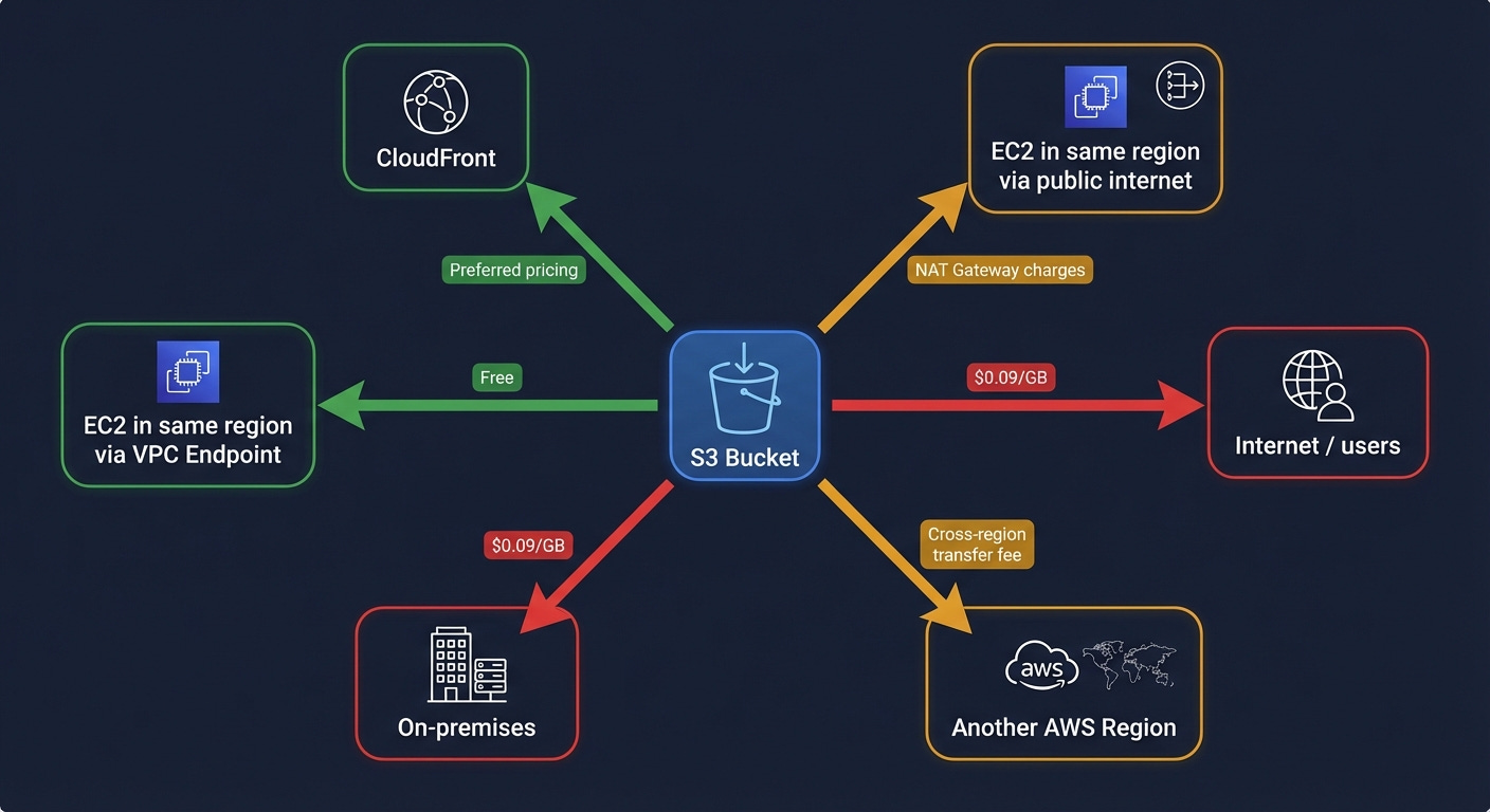
Egress to the internet: data leaving S3 to public internet destinations; costs $0.09 per GB in us-east-1 for the first 10 TB per month, scaling down slightly at higher volumes. Serving 100 TB of video from S3 to internet users is $9,000 per month in egress fees, before storage or API costs.
This is why CloudFront exists. CloudFront is AWS’s CDN (content delivery network) a global network of edge locations that cache content close to users. CloudFront has preferential pricing for S3 origin traffic and can serve cached content without generating per-request S3 API costs. For any application serving content to internet users, the S3 plus CloudFront architecture is almost always significantly cheaper than serving from S3 directly.
VPC Gateway Endpoints are free and almost nobody uses them. A VPC is a Virtual Private Cloud — AWS’s managed private network where your EC2 instances, Lambda functions, and other resources run. Normally, traffic from your VPC to S3 routes through the public internet, passing through a NAT Gateway; a managed service that translates private IP addresses to public ones for outbound internet access. NAT Gateway charges $0.045 per GB of data it processes. For a service like S3 that is internal to AWS, this is unnecessary.
A VPC Gateway Endpoint routes traffic from your VPC to S3 through AWS’s internal network, bypassing the public internet and the NAT Gateway entirely. It is free. It takes about two minutes to configure. It eliminates NAT Gateway data processing charges for all S3 traffic from your VPC, and it is generally faster than routing through the public internet. Create one in every VPC you own.
S3 Transfer Acceleration uses CloudFront’s edge network to accelerate uploads from geographically distant users. A user in Tokyo uploading to a bucket in us-east-1 routes through the nearest CloudFront edge location and then uses AWS’s private backbone network for the transoceanic portion, which is significantly more reliable and faster than routing over the public internet. The speed improvement for long-distance uploads is real: typically 50 to 500 percent faster. The cost is an additional per-GB fee on top of standard transfer rates. Worth modeling for user-facing applications where upload speed directly affects user experience.
Cross-region data transfer costs money whenever data moves between AWS regions. Replication, cross-region API calls, data pipelines that read from one region and write to another, all of these generate transfer costs. Design architectures to keep data co-located with the compute that processes it.
Observability: What Each Tool Actually Tells You
Server Access Logs write a log record for every request to the bucket into a destination bucket you specify. They are eventually consistent; delivery may be delayed by hours, and their format is a space-delimited text file that requires parsing. They are cheap: you pay for the storage of the log files. They tell you: what was requested, when, from what IP address, with what HTTP status code, how many bytes were transferred, and how long the request took. Use them for access pattern analysis, cost attribution by key prefix, and historical traffic investigation. Do not use them for real-time security monitoring, the latency is too high and the format is too primitive.
CloudTrail Data Events are the security monitoring tool. CloudTrail is AWS’s API audit service, it records every API call made to AWS services. Data Events extend this to S3 object-level operations: every GET, PUT, DELETE, and LIST call is captured with the full IAM principal identity (who made the call), the source IP address, the user agent, and the request parameters. Events appear within minutes. The cost is $0.10 per 100,000 events. At a bucket receiving 100 million requests per day, that is $100 per day in CloudTrail costs, $3,000 per month. Enable Data Events selectively on buckets containing sensitive, regulated, or high-value data. Not on every bucket by default.
Storage Lens is the fleet management tool. It aggregates metrics across all S3 buckets in all regions in your AWS organization; the organizational unit for managing multiple AWS accounts as a group. Storage Lens shows: total storage by class, object count, request rates, data retrieval volumes, replication status, and cost optimization recommendations. The free tier gives you 14 days of history. Storage Lens Advanced gives you 15 months of history, prefix-level metrics, and integration with S3 Tables for querying metrics with Athena. For organizations managing significant amounts of S3 storage, Storage Lens is where you find unexpected costs: buckets with large amounts of data sitting in S3 Standard that lifecycle rules should have tiered months ago, buckets with massive accumulations of unreferenced versioned objects, buckets generating large amounts of failed requests. It went from “nice dashboard” to “where I actually found that $20,000-per-month anomaly.”
EBS: Managed Disks
EBS is the right choice when you need block-level storage attached to a compute instance. Here is what you need to know to use it correctly.
Volume Types
gp3 is the current general-purpose volume and should be your default. It delivers 3,000 IOPS and 125 MB/s throughput as a baseline, with the ability to independently provision up to 16,000 IOPS and 1,000 MB/s regardless of volume size. IOPS stands for Input/Output Operations Per Second; a measure of how many read or write operations the disk can handle per second.
The “independent of size” part is the key improvement over the previous generation (gp2). With gp2, IOPS scaled automatically with volume size: 3 IOPS per GB. To get 3,000 IOPS, you needed a 1 TB volume even if you only had 50 GB of data. With gp3, you provision storage size and IOPS separately, paying only for what you actually need.
io2 Block Express is for workloads that need maximum performance: up to 256,000 IOPS, sub-millisecond latency. This is for high-performance databases (Oracle, SQL Server, SAP HANA) where storage latency is directly measurable in application response time. It supports Multi-Attach: an io2 volume can be attached to up to 16 Nitro-based EC2 instances simultaneously, all in the same AZ. This is the narrow exception to “block storage attaches to one instance at a time.” Use it for shared-disk database clusters that are explicitly designed for concurrent access.
st1 (Throughput Optimized HDD) is optimized for sequential reads and writes at high bandwidth; think Hadoop data nodes, log processing, data warehousing workloads that stream through large files. Lower cost per GB than gp3, lower IOPS, but high throughput for sequential access patterns.
sc1 (Cold HDD) is the cheapest EBS option, for data accessed very infrequently that still needs to be block-accessible. If you can use S3, use S3. If you need block storage and the data is accessed rarely, sc1.
Snapshots
EBS snapshots are incremental point-in-time copies stored in AWS-managed S3 infrastructure; not in your S3 buckets, but in S3 behind the scenes. The first snapshot copies the entire volume. Each subsequent snapshot copies only the blocks that changed since the previous snapshot. This makes them storage-efficient and fast to create after the initial snapshot.
Snapshots can be copied across regions for disaster recovery. A snapshot in us-east-1 can be copied to eu-west-1, and from that snapshot you can create a new EBS volume in the other region.
Fast Snapshot Restore is the option that eliminates the initialization penalty. When you create a new EBS volume from a snapshot, the data is lazily loaded from S3; each block is fetched from the snapshot on first access, which makes that first access significantly slower than subsequent accesses. Fast Snapshot Restore pre-initializes all blocks so the volume is immediately at full performance. It costs extra per AZ per snapshot enabled.
Cost check: gp3 storage is $0.08 per GB per month. A 1 TB gp3 volume is $80 per month plus $0.065 per provisioned IOPS above 3,000 and $0.04 per provisioned MB/s above 125. Snapshots are $0.05 per GB per month for the changed blocks stored. Old snapshots accumulate quietly. Automate snapshot lifecycle with AWS Data Lifecycle Manager or AWS Backup.
EFS and FSx: When You Actually Need a Shared Filesystem
EFS
EFS (Elastic File System) is managed NFS that scales automatically from gigabytes to petabytes. Multiple EC2 instances, across multiple AZs within a region, can mount it simultaneously and see the same directory tree.
Two performance modes: General Purpose gives lower latency and is right for all current workloads. Max I/O is a previous-generation mode designed for highly parallelized workloads, but AWS now recommends General Purpose for everything; Max I/O is not supported on One Zone file systems or file systems using Elastic throughput, and AWS’s own guidance says to always use General Purpose for faster performance.
Three throughput modes: Elastic automatically adjusts throughput to match your workload and you pay per gigabyte transferred; this is the default in the console today and the right choice for most workloads. Provisioned lets you specify a fixed throughput level that you pay for whether you use it or not, which makes sense when you have predictable high-throughput requirements. Bursting scales throughput proportionally with the amount of data stored in the filesystem, using a credit system similar to how burstable EC2 instances work; you accumulate burst credits during quiet periods and spend them during peaks. Bursting is the cheapest option for large file systems with intermittent high-throughput needs, but running out of burst credits during sustained heavy load is a real operational hazard.
EFS Infrequent Access is a storage class within EFS that moves files that have not been accessed for a configurable period (7, 14, 30, 60, or 90 days) to a cheaper storage tier. The file remains accessible with the same path; the tiering is transparent to applications. Enable it on any EFS filesystem where some files are accessed rarely.
Cost check: EFS Standard is $0.30 per GB per month. S3 Standard is $0.023. EFS costs thirteen times more. It is the right tool when you genuinely need shared filesystem semantics. It is not a general-purpose storage tier.
FSx
FSx for Windows File Server is a fully managed Windows filesystem that speaks SMB, integrates with Active Directory, and supports Windows-specific features: NTFS (the Windows filesystem format), Windows ACLs (Windows-native access control lists, different from S3 ACLs), DFS (Distributed File System, a Windows feature for unifying multiple network shares under a single namespace), and shadow copies (Windows’s version of point-in-time snapshots). Use this for Windows workloads that cannot be redesigned to use S3; legacy applications, applications that require a drive letter, applications built around Windows-specific filesystem behavior.
FSx for Lustre is a high-performance parallel filesystem that can sustain hundreds of GB/s of throughput. It was built for HPC (High Performance Computing) and ML training, workloads that need to feed enormous volumes of data to many compute nodes simultaneously. The native integration with S3 is notable: you link a Lustre filesystem to an S3 bucket, and files are lazily loaded from S3 into Lustre on first access. Your training job reads from Lustre at high speed; behind the scenes, Lustre fetches from S3. When the job finishes, results can be automatically written back to S3. You get the performance of a parallel filesystem with the durability and cost characteristics of S3 for long-term storage.
FSx for NetApp ONTAP is a managed version of NetApp’s enterprise NAS product. Multi-protocol access: NFS, SMB, and iSCSI simultaneously. Snapshots, cloning, thin provisioning; the full enterprise NAS feature set. The most relevant recent development: ONTAP can now expose file data through S3 Access Points, making it readable by services like Bedrock (AWS’s managed AI service), SageMaker (AWS’s ML platform), and Athena (AWS’s SQL query service) as if it were native S3 data. If you have an organization with significant existing NAS infrastructure that you want to connect to AI/ML services without migrating all the data first, FSx for ONTAP with S3 Access Points is the bridge.
Storage for AI and ML
AI and ML workloads have storage requirements that differ from traditional applications in three specific ways: they read the same data many times during training, they need to read at very high throughput, and they produce large amounts of intermediate output that needs cheap storage. Each of these requirements maps to a specific set of choices.
S3 as Data Lake Backbone
The canonical ML data pipeline looks like this: raw data arrives in S3, gets processed into training datasets (also stored in S3), is used to train a model (reading from S3), and the trained model artifacts are stored back in S3. Every step uses S3 as the persistence layer. Compute is ephemeral; it runs, does its work, and terminates. S3 is the durable record of everything that happened.
For training data ingestion, the key technique is byte-range GETs. Instead of downloading entire Parquet or TFRecord files, your training framework requests specific byte ranges. Multiple training workers can read different portions of the same large file in parallel without storing multiple copies. PyTorch’s DataLoader and TensorFlow’s tf.data support this natively. The practical effect: you can saturate GPU compute with data ingestion without paying for multiple copies of large training datasets.
For distributed training checkpoints, periodic saves of the model’s state during training, so a failure does not lose hours of work, write directly to S3 from training workers rather than to local disk first. Use multipart upload for checkpoint files over a few hundred MB; it is dramatically faster. Keep checkpoints in the same region as your training cluster to minimize latency and eliminate cross-region transfer costs.
S3 Tables for Feature Stores
A feature store is a database of pre-computed features (structured inputs to ML models) that gets reused across multiple model training runs and real-time inference requests. The problem it solves: feature computation is expensive. If five different models all need the same features derived from your user behavior data, you want to compute those features once and store them rather than recomputing for each model.
S3 Table Buckets with Iceberg format are a natural fit for the offline feature store; the portion used for training. Iceberg’s partition pruning makes queries like “give me all feature values for user IDs in this training batch” efficient without scanning the entire table. Iceberg’s append-only write model aligns with how feature values are generated: new values get appended, old values get retained for historical training runs.
The comparison with SageMaker Feature Store, AWS’s managed feature store service: SageMaker Feature Store provides both an offline store (backed by S3 and Glue) and an online store (backed by a fast, low-latency cache) for real-time inference. S3 Tables with Athena is significantly cheaper and more query-flexible for the offline use case. For real-time inference where you need sub-millisecond feature retrieval, SageMaker Feature Store’s online store is the right tool. Use both: S3 Tables for training data access, SageMaker Feature Store’s online store for real-time serving.
S3 Vectors for RAG Pipelines
The architecture for a RAG system built on S3 Vectors:
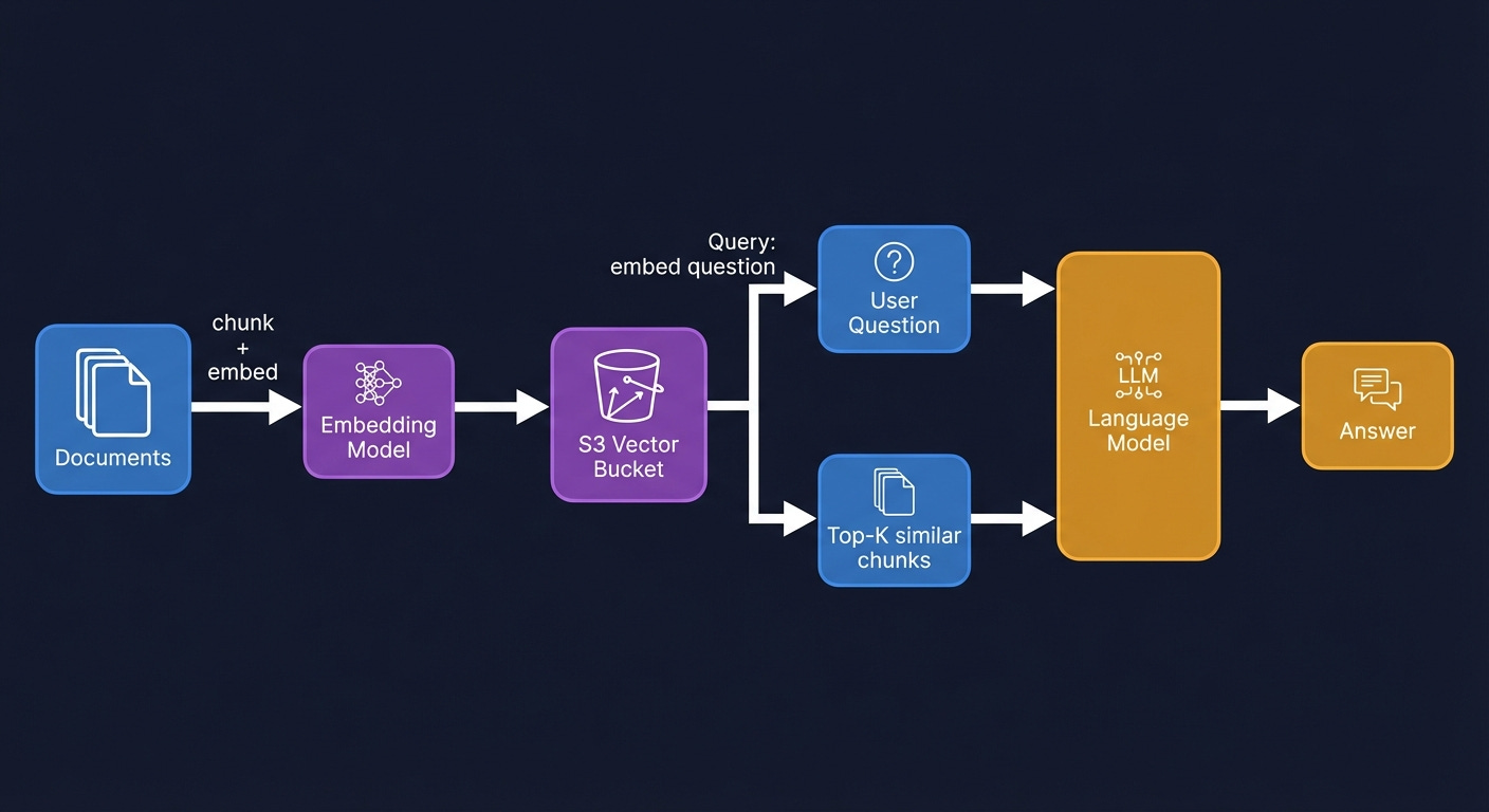
First, document ingestion. Process your documents; chunk them into segments of a few hundred tokens each, and generate an embedding for each chunk using an embedding model. Bedrock provides embedding models; you can also use OpenAI’s embedding API or run open-source models. Store each embedding in a Vector Bucket index. Store the original document chunks in a standard S3 bucket.
Second, query time. The user submits a question. Generate an embedding of the question using the same embedding model. Run a nearest-neighbor search against the Vector Bucket index. The index returns the keys of the k most semantically similar document chunks. Retrieve those chunks from standard S3. Include them as context in the prompt to your language model.
The critical tuning parameter is k; how many chunks to retrieve. Too small and you miss relevant context. Too large and you fill the model’s context window with noise that degrades response quality. Start with k=5, measure retrieval quality against a human-labeled evaluation set, and adjust.
When to use OpenSearch instead: if you need hybrid search combining vector similarity with keyword search, aggregations, faceted filtering, or consistently sub-100ms latency at high query volume. S3 Vectors supports metadata filtering in queries; you can filter by category, date, author, or any attribute alongside the vector similarity search, but OpenSearch’s query model is richer for applications that need more than nearest-neighbor retrieval.
When to use Bedrock Knowledge Bases instead: if you want the entire ingestion, chunking, embedding, and retrieval pipeline managed for you, Bedrock Knowledge Bases ingests documents from S3 and handles everything through a single API call. The tradeoff is flexibility; you control fewer parameters. Start with Knowledge Bases for prototyping; graduate to a custom Vector Bucket pipeline when you need to tune retrieval quality or manage costs at scale.
S3 Metadata for Data Cataloging
At scale, the hardest problem in ML operations is often not the model. It is knowing what data you have. Which training datasets were used for which model versions? Which datasets have been validated for quality? Where is the most recent version of the customer behavior feature set?
S3 Metadata solves the discovery problem at scale. Attach tags to your objects that encode dataset metadata: dataset=customer_reviews, version=2024Q4, quality_validated=true, processing_stage=cleaned. S3 Metadata indexes these tags automatically. Query with Athena: “find all objects tagged as customer reviews data from 2024 that passed quality validation.” The query returns in seconds, regardless of how many objects are in the bucket.
This is the foundation of a lightweight data catalog without additional managed services. It is not a replacement for a full ML metadata management system; tools like MLflow or SageMaker Experiments track model training runs, hyperparameters, and evaluation metrics. It is the complement that handles the storage discovery layer.
Getting Data In: Migration and Movement
The guide covers what to use and when. It has not covered how to actually move data there. That is a real gap for anyone starting from on-premises infrastructure or reorganizing data that already exists in AWS.
Moving data from on-premises to S3 depends on how much of it there is and how fast your network is. For datasets under a few terabytes, the AWS CLI’s s3 sync command handles it: it compares the source and destination, transfers what is missing, and is resumable. For larger datasets, AWS DataSync is a managed transfer service that handles scheduling, monitoring, retries, and data integrity verification automatically. It is significantly faster than running sync commands manually because it parallelizes transfers aggressively and does not require you to manage the transfer process.
For very large datasets (petabytes or tens of petabytes), AWS Snowball is the answer. AWS ships you a physical device, you load your data onto it locally, ship it back, and AWS ingests it into S3. Transferring a petabyte over a 1 Gbps internet connection takes roughly 100 days. Shipping a Snowball device takes about a week. The economics are obvious at that scale.
Moving data between S3 storage classes can happen in two ways. Lifecycle rules handle it automatically going forward based on object age. For existing data you want to reclassify immediately; moving a large cold dataset from Standard to Glacier because you just realized it has not been accessed in a year, S3 Batch Operations is the right tool. Create an inventory of the objects to reclassify, define the storage class change as the operation, run the job. It handles millions of objects in parallel without you writing any code.
Moving data between S3 buckets or regions uses CopyObject for individual objects, s3 sync for directory-style transfers between buckets, and S3 Batch Operations for bulk copies. Cross-region copies generate data transfer costs. Same-region copies within the same account do not. If you are reorganizing your bucket structure or consolidating data before enabling lifecycle rules, model the transfer costs before running the job.
A Unified Cost Model
Rather than making cost a separate section that people skip, here is the unified framework for thinking about storage costs across everything above.
All storage costs have four components: storage (per GB per month, by storage class), requests (per API operation), retrieval (per GB for tiered classes that charge for it), and transfer (per GB for egress and cross-region traffic). Every service has all four. They show up on your bill in different proportions depending on your access patterns.
The common mistakes, in rough order of frequency:
Storing everything in Standard when it should be tiered. Run an S3 Inventory, query it with Athena, find all objects not accessed in the last 90 days. That cohort multiplied by the difference between Standard and Glacier Instant rates is your monthly savings from one lifecycle rule.
Ignoring retrieval costs when choosing IA or Glacier tiers. If you access your IA data more than roughly once a month, the retrieval fees exceed the storage savings and Standard is actually cheaper. Model your retrieval patterns before moving data to lower tiers.
Forgetting to set a lifecycle rule for incomplete multipart uploads. This is a free savings. Set it on every bucket.
Not using VPC Gateway Endpoints. Also free. Set them in every VPC. The NAT Gateway cost savings are immediate.
Enabling SSE-KMS on high-request-rate buckets without modeling the KMS cost. KMS fees can exceed storage fees at scale. Use SSE-S3 unless you have a specific requirement for KMS.
Enabling CloudTrail Data Events on every bucket by default. At $0.10 per 100,000 events, a busy bucket generates meaningful CloudTrail costs. Enable selectively.
Not setting lifecycle rules for versioned objects. Versioning without expiration rules is a silent cost that compounds forever.
The pattern in all of these: AWS makes the zero-configuration path easy, and the cost-optimized path requires active choices. Each of the above items is a choice you have to make consciously. None of them are configured correctly by default.
The Full Mental Model
If there is one thing to take away from this guide, it is this: storage in AWS is a spectrum, not a menu.
At one end, you have block storage (EBS) which is a disk attached to one machine, fast and flexible, exactly like the storage you had before the cloud existed. It is the right choice when your software expects a disk and cannot be redesigned otherwise.
In the middle, you have file storage (EFS and FSx) which is a shared filesystem over the network. Multiple machines can use it simultaneously. It is the right choice when multiple compute nodes need concurrent filesystem access to the same data, and when that access pattern cannot be redesigned around object storage.
At the other end, you have object storage (S3) which is a distributed key-value store accessible over HTTP. Nothing is locked. Nothing is attached. Thousands of machines can read and write independently. It is the right choice for everything that can be modeled as “store a thing, retrieve a thing by name,” which is more of your data than you probably think.
S3 is now four services within that category: general purpose for the broad case, directory buckets for throughput-sensitive single-AZ workloads, table buckets for analytics and Iceberg-format data, and vector buckets for AI retrieval workloads. Most applications use general purpose buckets most of the time. The other three appear when a specific use case demands them.
The features layered on top of S3; storage classes, lifecycle rules, versioning, encryption, event notifications, Access Points, replication, Batch Operations, each exist because someone at scale ran into a problem and AWS built an answer. Every feature is a solution to a real production problem. Understanding the problem it was designed to solve makes the feature obvious rather than an entry on a list to be memorized.
Twenty years in, and the number keeps going up. Five hundred trillion objects. The service that got cheaper and more capable while everything else got more expensive. They called it Simple. They were wrong about that, but they were right about the rest.